Depth Anything 3：从任意视角恢复视觉空间

论文：Depth Anything 3: Recovering the Visual Space from Any Views
简称：DA3 / Depth Anything V3
arXiv：2511.10647
论文地址：arXiv 2511.10647

这篇论文解决什么问题

Depth Anything V1 / V2 主要是强大的单目深度模型：

single image -> dense depth

Depth Anything 3 把问题扩大到：

any number of views
with or without camera poses
-> consistent depth
-> rays / camera geometry
-> point clouds / rendering / pose estimation

也就是说，它不只是“单目深度 V3”，而是试图把 Depth Anything 系列推进到任意视角视觉几何。

论文的核心主张是：

一个 plain transformer backbone，加上合适的 depth-ray 表示和 teacher-student 训练，就足以统一 any-view geometry。

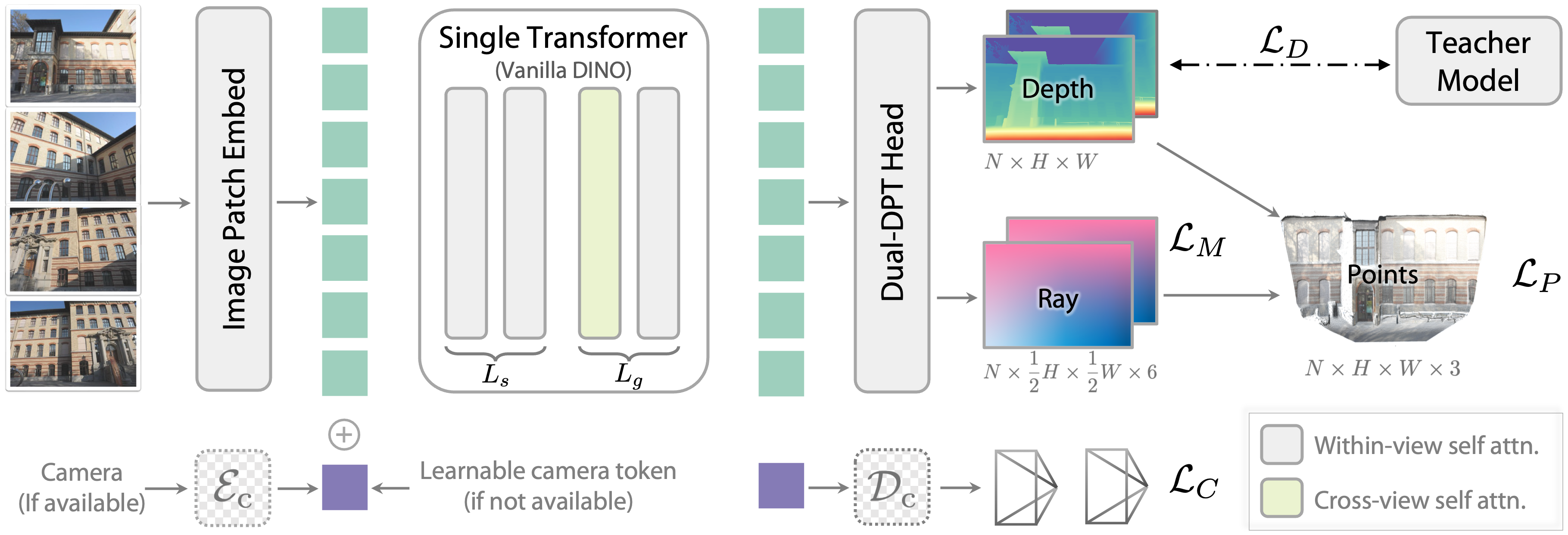
图源说明：来自 Depth Anything 3 arXiv 源码图，展示 DA3 的整体 pipeline。

一句话版本

DA3 可以记成：

images + optional camera poses
-> vanilla DINOv2-style transformer
-> adaptive cross-view self-attention
-> Dual-DPT head
-> depth maps + ray maps + optional camera head
-> point clouds / pose / depth / visual rendering

它和 VGGT / π³ 这些视觉几何模型很接近，但选择了一个更简洁的预测目标：

depth + ray

而不是直接堆很多输出头，或只回归 point maps。

输入与输出

输入是一组图像：

$$\mathcal{I} = \{\mathbf{I}_i\}_{i=1}^{N_v}$$

每张图：

$$\mathbf{I}_i\in\mathbb{R}^{H\times W\times 3}$$

当：

$$N_v=1$$

它就是单目深度估计。

当：

$$N_v>1$$

它可以是视频或多视角图像集合。

模型输出：

$$\mathcal{F}: \mathcal{I} \mapsto \{ \hat{\mathbf{D}}, \hat{\mathbf{R}}, \textcolor{gray}{\hat{\mathbf{C}}} \}$$

这里：

• $\hat{\mathbf{D}}$：depth map。
• $\hat{\mathbf{R}}$：ray map，论文里通常记作 ray map。
• $\textcolor{gray}{\hat{\mathbf{C}}}$：可选 camera pose head，主要为了推理方便。

从传统投影公式开始

如果已知相机内参：

$$\mathbf{K}_i$$

外参：

$$[\mathbf{R}_i\mid\mathbf{t}_i]$$

以及 depth：

$$\mathbf{D}_i(u,v)$$

像素：

$$\mathbf{p}=(u,v,1)^\top$$

对应 3D 世界点可写为：

$$\mathbf{X} = \mathbf{R}_i \left( \mathbf{D}_i(u,v) \mathbf{K}_i^{-1} \mathbf{p} \right) + \mathbf{t}_i$$

这就是你前面 pointmap 实验里的：

pixel -> camera ray -> depth -> 3D point

区别是 DA3 不希望显式依赖模型直接预测一个合法旋转矩阵，因为旋转矩阵需要满足正交约束：

$$\mathbf{R}^\top\mathbf{R}=\mathbf{I}$$

直接回归它并不舒服。

Depth-ray representation

DA3 用 per-pixel ray map 来隐式表达相机几何。

对每个像素：

$$\mathbf{p}=(u,v,1)^\top$$

定义一条 ray：

$$\mathbf{r}=(\mathbf{o},\mathbf{d}) \in\mathbb{R}^{6}$$

其中：

• $\mathbf{o}\in\mathbb{R}^3$：ray origin，也就是相机中心。
• $\mathbf{d}\in\mathbb{R}^3$：ray direction。

方向由：

$$\mathbf{d} = \mathbf{R} \mathbf{K}^{-1} \mathbf{p}$$

得到。论文中特别说：不对 $\mathbf{d}$ 做单位化，因为它的 magnitude 保留了 projection scale。

这样一个 3D 点可以直接由：

$$\mathbf{X} = \mathbf{o} + \mathbf{D}(u,v)\cdot\mathbf{d}$$

得到。

图源说明：根据 DA3 论文对 depth-ray representation 的公式描述重绘，非论文原图。

⭐ depth-ray 和 pointmap 有什么区别？

Pointmap 直接预测每个像素的 3D 点：

$$\mathbf{X}(u,v)\in\mathbb{R}^3$$

Depth-ray 则拆成：

$$\mathbf{D}(u,v)$$

和：

$$\mathbf{r}(u,v)=(\mathbf{o},\mathbf{d})$$

最后组合：

$$\mathbf{X}(u,v) = \mathbf{o} + \mathbf{D}(u,v)\mathbf{d}$$

直觉区别是：

pointmap：直接给结果点 X。
depth-ray：保留“从相机中心沿某条射线走多远”的几何结构。

Depth-ray 更接近针孔相机的投影过程，能同时表达：

场景结构：depth；
相机几何：ray origin + direction。

因此它比单纯 depth 更能做多视角几何，也比直接回归 rotation matrix 更容易训练。

如何从 ray map 恢复 camera 参数

ray map 的前 3 个通道是 ray origins：

$$\mathbf{R}_{map}(:,:,0:3)$$

后 3 个通道是 ray directions：

$$\mathbf{R}_{map}(:,:,3:6)$$

相机中心可以由所有 ray origin 平均得到：

$$\mathbf{o}_c = \frac{1}{H W} \sum_{h=1}^{H} \sum_{w=1}^{W} \mathbf{R}_{map}(h,w,:3)$$

为了恢复旋转和内参，论文构造一个 homography：

$$\mathbf{H} = \mathbf{K}\mathbf{R}$$

对于 canonical camera：

$$\mathbf{K}_I=\mathbf{I}$$

像素方向就是：

$$\mathbf{d}_I=\mathbf{p}$$

目标 ray direction 应满足：

$$\mathbf{d}_{cam} = \mathbf{K}\mathbf{R}\mathbf{d}_I = \mathbf{H}\mathbf{p}$$

于是求：

$$\mathbf{H}^* = \arg\min_{\lVert\mathbf{H}\rVert=1} \sum_{h=1}^{H} \sum_{w=1}^{W} \left\lVert \mathbf{H}\mathbf{p}_{h,w} \times \mathbf{R}_{map}(h,w,3:) \right\rVert$$

这是 DLT 可以求的 least-squares 问题。

得到：

$$\mathbf{H}^*$$

后，因为：

$$\mathbf{K}$$

是上三角矩阵，而：

$$\mathbf{R}$$

是正交矩阵，可以用 RQ decomposition 分解：

$$\mathbf{H}^* = \mathbf{K}\mathbf{R}$$

从而恢复 intrinsics 和 rotation。

⭐ 为什么 DA3 还要加一个 optional camera head？

理论上，ray map 已经包含相机信息，可以从 ray directions 恢复：

camera center
rotation
intrinsics

但这个恢复过程要做：

平均 ray origin；
构造 DLT；
求 homography；
RQ decomposition。

推理时会有额外计算。

所以 DA3 增加一个轻量 camera head：

$$\mathcal{D}_C$$

它只处理每个 view 的 camera token，预测：

$$\mathbf{c} = (\mathbf{t},\mathbf{q},\mathbf{f}) \in\mathbb{R}^{9}$$

其中：

• $\mathbf{t}\in\mathbb{R}^3$：translation。
• $\mathbf{q}\in\mathbb{R}^4$：rotation quaternion。
• $\mathbf{f}\in\mathbb{R}^2$：FOV / focal 相关参数。

论文说这个 head 的计算成本可以忽略，约为主干的 0.1%。

因此 camera head 不是因为 depth-ray 不够表达相机，而是为了实际使用更快更方便。

架构：plain transformer + adaptive cross-view attention

DA3 的主干是普通 ViT / DINOv2 风格 transformer。论文强调不需要复杂专用 3D 架构。

核心组件：

single transformer backbone
optional camera encoder
Dual-DPT prediction head

Single transformer backbone

设 transformer 总层数：

$$L$$

DA3 把层分为两组：

single-view layers
global / cross-view layers

前一部分只做单张图内部 self-attention。

后一部分通过 token rearrangement，让不同 view 的 tokens 可以交换信息。论文称它为 input-adaptive cross-view self-attention。

实验中采用：

$$L_{single}:L_{global}=2:1$$

也就是大约三分之二层做单图理解，三分之一层做跨视图推理。

⭐ 这和 VGGT 的 alternating attention 有什么关系？

VGGT 也交替使用：

frame-wise attention
global attention

DA3 的目标类似：既要保留单图局部/语义特征，又要让多视图 tokens 发生几何信息交换。

区别在于 DA3 更强调：

不改 backbone 架构；
通过 rearranging tokens 实现 input-adaptive cross-view self-attention；
最终只预测 depth + ray 这种更少、更统一的目标。

所以 DA3 和 VGGT 的关系可以理解为：

VGGT：多任务头很强，输出 cameras/depth/pointmaps/tracks。
DA3：主干尽量 plain，目标压缩到 depth-ray，再用 teacher-student 保细节。

⭐ DA3 是否说明 VGGT / π³ 的 AA Attention 整体冗余？

有这个迹象，但不能直接得出“AA Attention 整体冗余”的结论。 更准确地说，DA3 说明：VGGT / π³ 中固定、深层的“逐帧注意力—全局注意力交替堆叠”，可能不是实现多视角几何推理的唯一方式，其中确实存在结构和计算上的冗余。

但 DA3 并没有舍弃跨视角 attention。它仍然使用 Transformer self-attention，并引入 input-adaptive cross-view self-attention。DA3 舍弃的是 VGGT 式固定 AA 堆栈，而不是跨视角信息交互本身。

1. VGGT / π³ 的 AA 做什么？

VGGT 的 aggregator 交替执行：

Frame Attention -> Global Attention -> Frame Attention -> Global Attention -> ...

• Frame Attention：在单张图像内部通信，建模局部结构和单图上下文。
• Global Attention：让所有视图的 token 交换信息，完成跨视图匹配与对齐。

因此，AA 显式拆分了两种职责：

within-view reasoning + cross-view reasoning

VGGT 使用 DINO 特征作为初始图像 token，再经过较深的 AA aggregator；π³ 基本沿用了这种思路，但减少了层数，并去除了会破坏视图排列等变性的 reference-view 设计。AA 并不是无缘无故存在的，它确实把单图建模和跨图几何推理分开处理。

2. DA3 实际上改变了什么？

DA3 的观点不是“跨视角 attention 不需要”，而是“不需要专门构造一套固定的、很深的 alternating-attention aggregator”。一个经过改造的普通 DINO-style Transformer，也可以同时承担单图表征和多图推理。

可以粗略对比为：

VGGT: DINO encoder -> 显式 AA aggregator F,G,F,G,... -> 多个任务头
DA3:  DINO-style Transformer -> 自适应单图/跨图 attention -> depth-ray head

DA3 通过 token rearrangement，让 self-attention 根据输入情况进行跨视图交换，因此更像是把 encoder 与 aggregator 融合为一个统一 backbone，而不是删除 aggregator 的功能。

3. 为什么 DA3 可以使用更简单的结构？

这不只是 attention 设计不同，输出目标也被简化了。

VGGT 同时预测：

K, R, t, depth, point map, tracking feature

这些任务对表示的要求不同：camera token 需要图像级全局信息，point/depth head 需要高分辨率局部信息，tracking 需要稳定的跨视图对应关系。因此 VGGT 的 AA stack 要为多个异质任务共同构造中间表示。

DA3 主要统一为：

$$\text{depth} + \text{ray map}$$

然后通过

$$\mathbf{P}_w = \mathbf{t} + D\mathbf{d}$$

恢复世界坐标点和相机相关几何。这样 backbone 不必同时服务多个相互独立的输出空间。

所以 DA3 的成功可能同时来自：

更合适的表示目标 + 更强的数据与蒸馏 + 更简洁的 attention 组织

不能只归因于“AA 没用”。

4. 后续研究是否发现 AA 中存在冗余？

确实有较强迹象。对 VGGT 和 π³ 的层级分析表明：早期 global 层可能尚未形成有意义的跨视图对应，中间 global 层主要完成跨视图对齐，后期 global 层通常只做小幅细化。

因此，一些改进方法尝试把早期部分 global attention 替换为 frame attention，并稀疏化其余 global attention，在基本保持甚至略微提升精度的情况下获得最高约 8-10x 的加速。另一些工作发现，dense global attention 的有效关系主要集中在少量具有几何对应意义的 token 对上，因此 block-sparse attention 也可以在较小精度损失下减少计算。

这说明：

AA 中的 global attention 确实不是每一层、每一个 token 都同等必要。

但这仍然不等于“整个 AA 机制冗余”。

5. 哪些部分更可能冗余？

可以拆成三类：

层数冗余。 VGGT 的每个阶段都固定插入 global attention，但真正负责建立 correspondence 的可能只是中间若干层。也就是说，在 G_1, G_2, ..., G_24 中，只有部分层可能是关键跨视图推理层。

token 交互冗余。 Dense global attention 的计算量近似为

$$O((NHW)^2)$$

但真实跨视图 correspondence 往往是稀疏的。大量 token 对来自无重叠区域、天空和墙面等低信息区域、完全不相关的视图，或同一物体上重复而低价值的局部。

功能重复。 DINO 特征本身已经包含较强的语义和空间结构。如果 AA 中许多 frame-attention 层只是重复构造单图特征，那么 DINO backbone 与 AA 的 frame branch 之间可能存在功能重叠。DA3 直接把 DINO-style Transformer 微调为几何模型，可能减少了“单图 encoder + 再次进行大量单图 attention”的重复。

6. DA3 能证明 AA 在所有场景下都多余吗？

不能。至少有三个变量没有完全控制：

• 训练数据和监督不同。 DA3 使用 teacher-student 训练和大规模几何伪标签，更强的监督可能补偿了结构简化。公平比较应保持数据、参数量、输出目标和训练 recipe 一致，只改变 attention 组织。
• 输出任务不同。 VGGT 还承担 tracking、camera、depth、point map 等多任务；DA3 的核心目标更集中。不能因为 depth-ray 模型不需要 VGGT 式 AA，就推断多任务模型也不需要。
• 场景规模和视角条件不同。 在几十到几百视图、低重叠、大基线、强重复纹理或大范围场景中，显式跨视图聚合仍可能有优势。DA3 仍然保留 cross-view attention，本身就说明单纯逐图 DINO 不足以完成这些任务。

7. 最准确的结论

可以分成三级：

1. 可以确定： VGGT 式固定而深的 AA 不是实现强多视角几何的必要条件。
2. 有较强证据： AA 中大量 global 层和 dense token 交互存在冗余，尤其是早期、晚期 global attention，以及没有真实对应关系的 token 对。
3. 尚不能确定： 跨视图 attention 本身是冗余的。DA3 并未去掉它，只是换成了更自适应、更融合的实现形式。

因此，更严谨的表述是：

DA3 表明专门化、固定重复的 AA 架构可能存在过度设计；它并没有表明跨视图 attention 不重要，而是表明跨视图推理可以更简洁、更自适应地整合进普通 ViT。

8. 对 Pi3X hook 实验的启发

你已经能够 hook aggregator 的中间层，最值得验证的问题是：哪些 AA 层真正产生了跨视图几何，哪些层只是在重复加工特征？可以逐个 global 层测量：

cross-view correspondence accuracy
relative-pose linear-probe accuracy
point-map consistency
attention entropy / effective attended tokens

还可以做逐层干预：

global attention -> frame-only
global attention output -> 0
skip one global block

然后观察 pose、point map 和 depth 的下降幅度。一个合理的预期是：早期层偏向单图语义与局部结构，中间 global attention 对 correspondence 和 pose 最关键，后期层更多负责 depth/point refinement，但并非每一组 AA 都同样重要。

⭐ Pi3 camera 输出与 DA3 ray 输出的关系

⭐ Pi3 的 camera 与 DA3 的 ray 到底有什么区别？

1. Pi3 的 camera 输出是什么？

Pi3（类似 VGGT）通常为第 $i$ 个视角预测：

$$\left(\mathbf{K}_i,\mathbf{R}_i,\mathbf{t}_i\right)$$

常见定义是：

$$\mathbf{T}_{c\rightarrow w}= \left[\mathbf{R}_i\mid\mathbf{t}_i\right], \qquad \mathbf{P}_w=\mathbf{R}_i\mathbf{P}_c+\mathbf{t}_i$$

其中：

• $mathbf{R}_i$ 表示 camera 坐标系到 world 坐标系的旋转；
• $mathbf{t}_i$ 是 camera center 在 world 坐标系中的位置；
• $mathbf{K}_i$ 是相机内参，例如

$$\mathbf{K}= \begin{bmatrix} f_x&0&c_x\\ 0&f_y&c_y\\ 0&0&1 \end{bmatrix}.$$

因此 Pi3 的 camera 输出是一个图像级全局变量：一张图对应一组 $(\mathbf{K},\mathbf{R},\mathbf{t})$。

2. DA3 的 ray 输出是什么？

DA3 对每个像素 $(u,v)$ 输出一个 ray：

$$\mathbf{M}(u,v)=\left(\mathbf{t}(u,v),\mathbf{d}(u,v)\right)$$

其中：

• $mathbf{t}(u,v)$ 是该像素射线的 origin；
• $mathbf{d}(u,v)$ 是该像素射线的 direction；
• $D(u,v)$ 是该像素的 depth。

最终点由：

$$\mathbf{P}_w(u,v)=\mathbf{t}(u,v)+D(u,v)\mathbf{d}(u,v)$$

得到。

3. 数学上二者有什么关系？

如果给定 Pi3 的一个像素：

$$\tilde{\mathbf{p}}=[u,v,1]^T$$

先由内参反投影到 camera 坐标系：

$$\mathbf{P}_c=D\mathbf{K}^{-1}\tilde{\mathbf{p}}.$$

再变换到 world 坐标系：

$$\begin{aligned} \mathbf{P}_w &=\mathbf{R}\left(D\mathbf{K}^{-1}\tilde{\mathbf{p}}\right)+\mathbf{t}\\ &=\mathbf{t}+D\left(\mathbf{R}\mathbf{K}^{-1}\tilde{\mathbf{p}}\right). \end{aligned}$$

因此可以识别出：

$$\mathbf{d}(u,v)=\mathbf{R}\mathbf{K}^{-1}\tilde{\mathbf{p}}, \qquad \mathbf{t}(u,v)=\mathbf{C}=\mathbf{t}.$$

在理想针孔相机模型下，Pi3 的 $(\mathbf{K},\mathbf{R},\mathbf{t})$ 可以生成 DA3 所需的 $(\mathbf{t}(u,v),\mathbf{d}(u,v))$。

4. 为什么又说 DA3 不直接预测 camera？

关键在于表示粒度不同。

Pi3 预测一组全局 camera 参数：

one image -> K, R, t

例如一张图只需要若干个内参、旋转和平移参数。

DA3 则为每个像素预测 ray：

one image -> H x W x 6 ray values

对于 640 x 480 图像，ray 本身就包含约 $640\times480\times6$ 个数。它表面上输出更多，但不要求所有像素严格服从同一个全局 pinhole camera 参数化。

5. 二者的关键区别是约束方式

Pi3 camera 需要满足显式几何约束：

$$\mathbf{R}^T\mathbf{R}=\mathbf{I},$$

并且 $mathbf{K}$ 通常是上三角内参矩阵。否则输出就不是合法的 camera。

DA3 ray 直接预测每个像素的三维方向，例如：

$$\mathbf{d}=(0.5,0.2,1.0).$$

它不必显式保证所有像素方向都能由同一个 $mathbf{R}\mathbf{K}^{-1}[u,v,1]^T$ 生成，也不必显式保证所有 ray origin 相同。换句话说：

Pi3 camera：低维、全局、强约束
DA3 ray：高维、逐像素、弱显式约束

这也是 DA3 更灵活、但表示量更大的原因。DA3 并不是“没有相机几何”，而是把一部分 camera 几何从全局参数化改成了逐像素 ray field。

Camera condition injection

DA3 可以处理两种输入：

没有已知相机参数
有已知相机参数

如果有 camera parameters：

$$(\mathbf{K}_i,\mathbf{R}_i,\mathbf{t}_i)$$

就通过 camera encoder：

$$\mathbf{c}_i = \mathcal{E}_c (\mathbf{f}_i,\mathbf{q}_i,\mathbf{t}_i)$$

得到 camera token。

如果没有相机参数，就使用共享 learnable token。

这些 camera tokens 会和 patch tokens 拼接，并参与所有 attention。

Dual-DPT head

DA3 使用 Dual-DPT head 同时预测 depth 和 ray。

结构可以概括为：

backbone features
-> shared reassembly modules
-> depth fusion branch
-> ray fusion branch
-> depth output / ray output

论文的观点是：depth 和 ray 都来自同一组视觉特征，应该共享前面的 reassembly，但最后融合层分开，避免两个任务完全绑死。

⭐ 为什么不是直接多任务输出 depth + pointmap + camera 越多越好？

VGGT 这类模型有多个输出头：

camera
depth
point map
tracking features

多任务能提供冗余监督，有时确实提升效果。但 DA3 认为冗余目标也会带来 entanglement：

各个任务之间可能互相牵制；
输出之间可能不完全一致；
训练和架构复杂度变高。

DA3 的 ablation 显示，depth + ray 已经是一个很强的最小目标组合。

实验中：

目标组合	HiRoom Auc3	HiRoom F1	ETH3D F1
depth + pcd + cam	9.1	12.8	60.4
depth + cam	10.8	16.5	48.0
depth + ray	48.7	60.3	65.4
depth + ray + cam	37.2	45.4	59.4

不过论文最终仍采用 depth + ray + cam，因为 camera head 推理更方便，计算成本很小，并且在部分数据集如 DTU、7Scenes、ScanNet++ 上更好。

Teacher-student learning

DA3 的训练数据来源很复杂：

real-world depth camera captures
3D reconstruction / COLMAP
synthetic data

问题是：真实世界深度常常噪声大、稀疏、不完整。直接训练会损失细节。

DA3 采用 teacher-student：

synthetic clean depth
-> train a strong monocular relative depth teacher
-> teacher predicts dense pseudo-depth for real-world images
-> align pseudo-depth with noisy/sparse metric depth using RANSAC scale-shift
-> train DA3 student with richer supervision

图源说明：根据 DA3 论文 teacher-student 训练范式重绘，非论文原图。

teacher 是单目 relative depth 模型，只在 synthetic data 上训练。它继承 DA2 的路线，但做了几项改变：

• 扩展合成数据规模，覆盖 indoor、outdoor、object-centric、in-the-wild。
• 从 scale-shift-invariant disparity 改成 scale-shift-invariant depth。
• 使用 exponential depth，增强近距离区分能力。
• 引入 normal loss、global-local loss、sky mask、object mask 等。

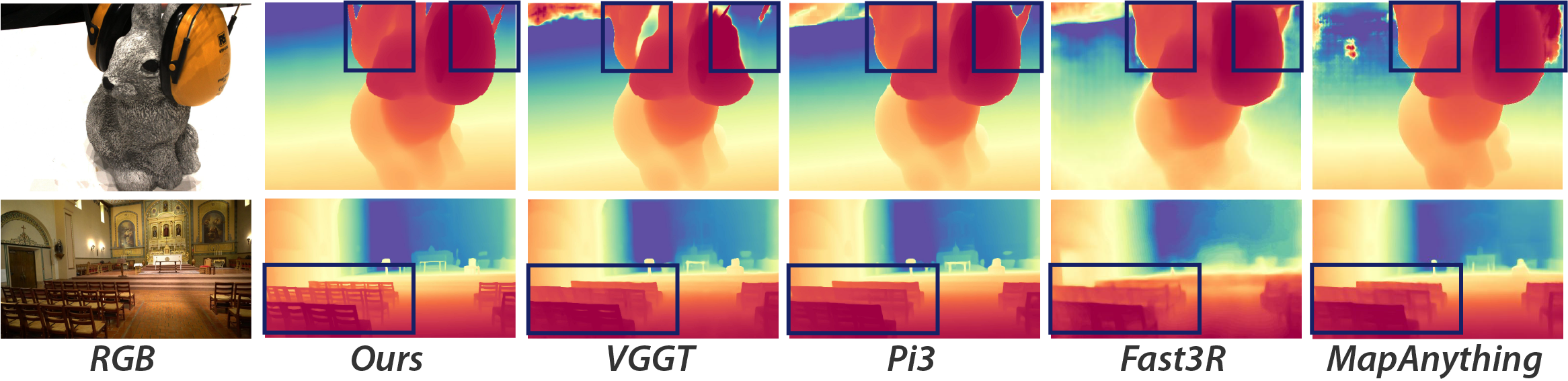
图源说明：来自 Depth Anything 3 arXiv 源码图，展示 depth 质量对比。

⭐ 为什么 teacher 用 synthetic data，而 student 还要用 real-world data？

synthetic data 的优点：

dense depth 干净；
相机参数准确；
几何标签完整；
能覆盖很多受控场景。

缺点：

外观和真实世界有 domain gap；
真实相机噪声、运动模糊、反光、遮挡更复杂。

real-world data 的优点：

真实外观分布；
真实相机和场景复杂性；
对泛化很重要。

缺点：

depth 可能稀疏；
COLMAP 点云可能缺区域；
RGB-D 传感器有噪声；
动态物体和反光表面会产生错误。

DA3 的折中是：

用 synthetic 训练一个几何细节更干净的 teacher；
再用 teacher 给 real-world data 补充密集细节；
同时用原始 noisy/sparse metric depth 做 scale-shift alignment，保住尺度和几何一致性。

训练目标

DA3 的模型输出：

$$\mathcal{F}: \mathcal{I} \mapsto \{ \hat{\mathbf{D}}, \hat{\mathbf{R}}, \textcolor{gray}{\hat{\mathbf{c}}} \}$$

训练前，ground-truth 信号会按一个共同尺度归一化。这个尺度定义为有效重投影 point maps 的平均 $\ell_2$ norm，用于稳定不同模态的 magnitude。

总 loss：

$$\mathcal{L} = \mathcal{L}_D(\hat{\mathbf{D}},\mathbf{D}) + \mathcal{L}_R(\hat{\mathbf{R}},\mathbf{R}) + \mathcal{L}_P (\hat{\mathbf{D}}\odot\mathbf{d}+\mathbf{o},\mathbf{X}) + \textcolor{gray}{\beta\mathcal{L}_C(\hat{\mathbf{c}},\mathbf{c})} + \alpha\mathcal{L}_{grad}(\hat{\mathbf{D}},\mathbf{D})$$

其中：

• $\mathcal{L}_D$：depth loss。
• $\mathcal{L}_R$：ray loss。
• $\mathcal{L}_P$：由 depth + ray 组成 point cloud 后的 point loss。
• $\mathcal{L}_C$：optional camera loss。
• $\mathcal{L}_{grad}$：depth gradient loss，约束边缘和局部平滑。

论文设置：

$$\alpha=1,\quad \beta=1$$

depth loss 是 confidence-aware L1：

$$\mathcal{L}_D = \frac{1}{Z_\Omega} \sum_{p\in\Omega} m_p \left( D_{c,p} \left| \hat{D}_p-D_p \right| - \lambda_c\log D_{c,p} \right)$$

gradient loss：

$$\mathcal{L}_{grad} = \lVert \nabla_x\hat{\mathbf{D}} - \nabla_x\mathbf{D} \rVert_1 + \lVert \nabla_y\hat{\mathbf{D}} - \nabla_y\mathbf{D} \rVert_1$$

这个 loss 会帮助保留深度边缘，同时让平面区域更平滑。

训练细节

DA3 使用公开学术数据集训练。论文列出了用于 pose-geometry training 的 21 个数据源，包括 ArkitScenes、BlendedMVS、CO3D-v2、DL3DV、HyperSim、MapFree、MegaDepth、Objaverse、ScanNet++、TartanAir、Trellis、vKITTI2、WildRGBD 等。

主要训练设置：

项目	设置
训练硬件	128 H100 GPUs
步数	200k steps
warm-up	8k steps
peak lr	$2\times10^{-4}$
base resolution	$504\times504$
view 数量	$504\times504$ 时从 2 到 18 均匀采样
batch	动态调整，保持 token count 近似恒定
teacher 切换	120k steps 后从 GT depth 过渡到 teacher labels
pose conditioning	训练时以 0.2 概率激活

选择 504 作为基础尺寸的原因是它能被 2、3、4、6、9、14 整除，适配常见照片宽高比和 patch size。

实验结论

Camera pose

DA3 在多个 pose benchmark 上超过 VGGT、π³、MapAnything 等方法。部分结果：

方法	参数量	HiRoom Auc3	ETH3D Auc3	DTU Auc3	ScanNet++ Auc3
Pi3	0.96B	67.0	35.2	62.5	50.7
VGGT	1.19B	49.1	26.3	79.2	62.6
DA3-Giant	1.10B	80.3	48.4	94.1	85.0
DA3-Large	0.36B	58.7	32.2	70.2	60.2

一个明显现象是：DA3-Giant 在多数数据集上 pose accuracy 很强，DA3-Large 参数量只有 0.36B，但也能接近或超过许多更大模型。

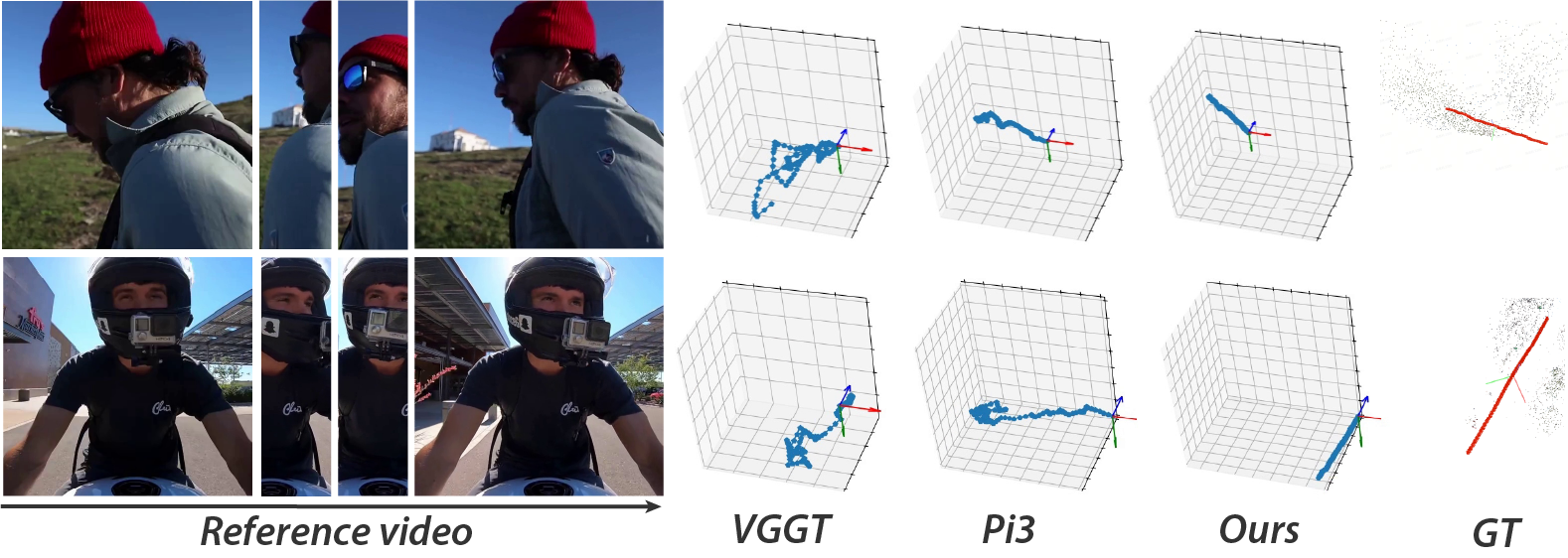
图源说明：来自 Depth Anything 3 arXiv 源码图，展示 camera trajectory 估计质量。

Reconstruction

重建指标中，论文对除 DTU 外的数据集报告 F-score，对 DTU 报 Chamfer Distance。

部分结果：

方法	HiRoom F1 w/o pose	ETH3D F1 w/o pose	DTU CD w/o pose	ScanNet++ F1 w/o pose
Pi3	75.8	72.7	3.28	63.1
VGGT	56.7	57.2	2.05	66.4
DA3-Giant	85.1	79.0	1.85	77.0
DA3-Large	69.5	65.8	2.08	67.9

如果提供 ground-truth pose，DA3 也可以利用 pose conditioning 提升部分数据集结果。

模型规模和速度

论文报告在 A100 80GB 上测试最大输入图像数量，并用 32 张图场景测每图速度。

模型	最大图像数	速度
VGGT reference	400-500	34.1 FPS
DA3-Giant	900-1000	37.6 FPS
DA3-Large	1500-1600	78.37 FPS
DA3-Base	2100-2200	126.5 FPS
DA3-Small	4000-4100	160.5 FPS

这个表说明 DA3 的 plain transformer + depth-ray 设计在长序列上更可扩展。

Monocular depth

DA3 还给出了单目 student depth 结果。以 $\delta_1$ 为指标：

方法	KITTI	NYU	SINTEL	ETH3D	DIODE
DA2	94.6	97.9	77.2	86.5	95.2
DA3 mono-student	97.1	98.0	82.3	98.8	96.5

这说明 DA3 的 teacher-student 训练不仅服务多视图几何，也反过来提升单目深度质量。

Ablation：哪些设计真的有用

架构设计

论文比较了：

• proposed architecture；
• VGGT style；
• full alternating attention；
• 去掉 Dual-DPT；
• 去掉 teacher；
• 有无 pose conditioning。

关键结果是：proposed architecture 在多数 benchmark 上比 VGGT-style 好很多。例如：

设计	HiRoom Auc3	ETH3D Auc3	DTU Auc3	ScanNet++ Auc3
Proposed Arch.	39.2	21.0	45.8	30.3
VGGT Style	3.72	2.31	1.38	2.03
Full Alt.	24.7	13.1	44.6	27.7

这支持论文的观点：不是简单照搬 VGGT 的 attention 组织就够，DA3 的单图/跨图层比例和 token 重排方式很关键。

prediction target

最重要的 ablation 是预测目标组合：

目标	HiRoom Auc3	ETH3D Auc3	DTU Auc3	ScanNet++ F1
depth + pcd + cam	9.1	19.0	42.3	43.0
depth + cam	10.8	9.9	23.3	41.0
depth + ray	48.7	25.5	46.5	53.4
depth + ray + cam	37.2	22.3	56.3	56.5

结论：

depth + ray 是最核心的组合；
camera head 主要提供 practical convenience；
point cloud 直接回归不如 depth-ray 稳。

和 VGGT / π³ / MASt3R 的关系

方法	核心输出	关键设计	适合怎么理解
MASt3R	pointmaps + dense descriptors	3D-grounded matching	把 DUSt3R 变成强 matching engine
VGGT	cameras + depth + pointmaps + tracks	多任务几何 transformer	用 feed-forward 模型替代很多传统几何步骤
π³	local pointmaps + relative cameras	permutation-equivariant / reference-free	去掉 reference view bias
DA3	depth + ray + optional camera	minimal depth-ray target + teacher-student	用 depth-ray 统一任意视角几何

DA3 和 VGGT 最像，但它提出不同取舍：

VGGT：输出冗余 3D 属性，追求统一多任务。
DA3：把目标压缩成 depth-ray，靠简洁表示和强 supervision 做统一。

DA3 和 π³ 也不是同一个方向：

π³ 重点是输入顺序和 reference view bias；
DA3 重点是 depth-ray 表示、pose conditioning 和 teacher-student training。

我认为最关键的理解

DA3 的中心句可以写成：

depth 是结构，ray 是相机几何；
depth + ray 就能恢复 3D visual space。

这和你前面 pointmap 笔记中的关系正好对应：

pixel
-> camera ray
-> depth
-> 3D point

DA3 只是把这件事改成神经网络预测：

网络预测每个像素的 depth；
网络预测每个像素的 world ray；
二者组合得到一致 point cloud；
再从 ray map 或 camera head 得到 pose。

⭐ DA3 为什么叫 Recovering the Visual Space from Any Views？

因为它不限制输入形式：

单张图；
视频；
多视角图像集合；
有相机参数；
没有相机参数。

在这些情况下，它都试图输出一致的：

depth maps；
ray maps；
camera geometry；
point clouds。

所以它不是只做一张图的相对深度，而是试图从任意视角输入恢复一个可融合、可渲染、可估计 pose 的视觉空间。

读完后应该记住的公式

传统 depth + camera 到 3D：

$$\mathbf{X} = \mathbf{R}_i \left( \mathbf{D}_i(u,v) \mathbf{K}_i^{-1} \mathbf{p} \right) + \mathbf{t}_i$$

Depth-ray：

$$\mathbf{r} = (\mathbf{o},\mathbf{d}) \in\mathbb{R}^{6}$$

ray direction：

$$\mathbf{d} = \mathbf{R} \mathbf{K}^{-1} \mathbf{p}$$

point from depth-ray：

$$\mathbf{X} = \mathbf{o} + \mathbf{D}(u,v)\mathbf{d}$$

camera center from ray origins：

$$\mathbf{o}_c = \frac{1}{HW} \sum_{h,w} \mathbf{R}_{map}(h,w,:3)$$

training objective：

$$\mathcal{L} = \mathcal{L}_D + \mathcal{L}_R + \mathcal{L}_P + \textcolor{gray}{\beta\mathcal{L}_C} + \alpha\mathcal{L}_{grad}$$

个人总结

Depth Anything 3 最值得放在 VGGT 和 π³ 后面读。

VGGT 让你看到：

一个大模型可以直接输出 cameras、depth、pointmaps、tracks。

π³ 让你看到：

坐标系和 reference view 的选择会影响模型稳定性。

DA3 则强调：

如果预测目标选得足够几何化，depth + ray 就能把结构和相机运动统一起来。

这对后面理解多视角点云融合、ray map、depth-to-pointmap、pose estimation 都很直接。